Introduction
In the previous post, a simplified Fully Convolutional Network (FCN) was implemented by means of Chainer. Its accuracy is lower than that of the original FCN. In this post, I have remarkably improved the accuracy by the following modifications:
- The original implementation of the FCN is written with Caffe. Caffe supports a "CropLayer" which the original code uses. Unfortunately Chainer does not support layers corresponding to the "CropLayer." I have noticed, however, that the similar outcome is achieved by utilizing an argument "outsize" which is passed to a function "chainer.functions.deconvolution_2d." The use of the function allows my code to accept inputs of any size. In the previous post, an input was made square with 224$\times$224 in advance.
- In the previous post, I didn't understand the fact that an image with information on labels in VOC dataset is not RGB mode, but index one. Therefore, I spent time to implement a function by which RGB is converted to an integer value. In this post, an index image is read using index mode directly.
- The procedures of the construction of the original FCN is fcn32s $\rightarrow$ fcn16s $\rightarrow$ fcn8s. The accuracy of the FCN depends mostly on that of the fcn32s, and the contributions from the fcn16s and the fcn8s are at most 1%. Though I showed the implementation of the fcn8s in the previous post, in this post the code of the fcn32s is demonstrated.
- As a mini batch learning was employed in the previous post, "chainer.links.BatchNormalization" was able to be introduced. In this post, there is no room to introduce the normalization because of the use of a one-by-one learning.
- In the previous post, weights in deconvolutional layers were learned using "chainer.links.Deconvolution2D." In this post, the deconvolutional layers are fixed to the simple bilinear interpolation.
Learning Curve
The resultant learning curves are as follows:
Accuracy


Computation Environment
The same instance as the previous post, g2.2xlarge in the Amazon EC2, is used. As input images have various sizes, there is no choice but to run the one-by-one learning. The mini batch learning is not able to be used. It takes 3.5 days for the above learning curves to converge.
Dataset
Just as before, the FCN is trained on a dataset VOC2012 which includes ground truth segmentations. The number of images is 2913. I divided them by the split ratio 4:1. The former set of images corresponds to a training dataset, and the latter a testing one.
| number of train | number of test |
|---|---|
| 2330 | 583 |
As described above, all images are not resized in advance. The number of the categories is 20+1(background).
| label | category |
|---|---|
| 0 | background | 1 | aeroplane | 2 | bicycle | 3 | bird | 4 | boat | 5 | bottle | 6 | bus | 7 | car | 8 | cat | 9 | chair | 10 | cow | 11 | diningtable | 12 | dog | 13 | horse | 14 | motorbike | 15 | person | 16 | potted plant | 17 | sheep | 18 | sofa | 19 | train | 20 | tv/monitor |
Network Structure
The detailed structure of a network is as follows:

pool5. For simplicity, these layers are again removed. Under the assumption that an image is a square with 224 $\times$ 224, one side length of an image is written to a column "input" of the table shown above. It should be noticed that the FCN implemented in this post is actually permitted to accept inputs of any size. Each column of the table indicates:
- name: a layer name
- input: a size of an input feature map
- in_channels: the number of input feature maps
- out_channels: the number of output feature maps
- ksize: a kernel size
- stride: a stride size
- pad: a padding size
- output: a size of an output feature map
score-pool5 following pool5 is required. I refer to an output of score-pool5 as p5. The number of feature maps of p5 is equal to that of categories (21).
p5 back to input size, it is compared with a label image.

Implementation of Network
The network can be written in Chainer like this:
-- myfcn_32s_with_any_size.py -- By assigning a label of -1 to pixels on the borderline between objects, we can ignore contribution from those pixels when calculating
softmax_cross_entropy (see the Chainer's specification for details). Using an argument "ignore_label" passed to a function "F.accuracy" allows us to calculate the accuracy without contribution from pixels on the borderlines. The function "F.deconvolution_2d" shown from the 99th line to the 100th line upsamples p5 back to the input size.
Training
The script for training is as follows:
-- train_32s_with_any_size.py -- I used
copy_model and VGGNet.py described in the previous post.
The procedures shown in the script train_32s_with_any_size.py are as follows:
- make an instance of the type MiniBatchLoaderWithAnySize
- make an instance of the type VGGNet
- make an instance of the type MyFcn32sWithAnySize
- copy parameters of the instance of VGGNet to those of that of MyFcn32sWithAnySize
- select MomentumSGD as an optimization algorithm
- run a loop to train the net
mini_batch_loader_with_any_size.py is written like this:
-- mini_batch_loader_with_any_size.py --
The function
load_voc_label shown from the 91th line to the 96th line loads a label image using the index mode and replaces 255 with -1. To load all the training data on the GPU memory at a time causes the error "cudaErrorMemoryAllocation: out of memory" to occur. Therefore, only one pair of an image and a label is loaded every time a training procedure requires it. Prediction Results
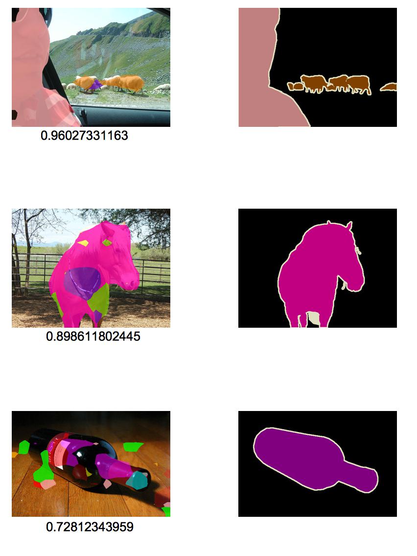
The left column shows prediction images overlaid on testing images. A value under each image indicates an accuracy which is defined as the percentage of the pixels which have labels classified correctly that are not on the borderlines between objects. The right column shows the ground truths.


Download
You can download tag 2016-07-09
0 件のコメント:
コメントを投稿